Tutorial 4: Key term extraction
Andreas Niekler, Gregor Wiedemann
2020-10-08
This tutorial shows how to extract key terms from document and (sub-)collections with TF-IDF and the log-likelihood statistic and a reference corpus. We also show how it is possible to hande multi-word units such as `United States’ with the quanteda package.
- Multi-word tokenization
- TF-IDF
- Log-likelihood ratio test
- Visualization
1 Multi-word tokenization
Like in the previous tutorial we read the CSV data file containing the State of the union addresses and preprocess the corpus object with a sequence of quanteda functions.
In addition, we introduce handling of multi-word units (MWUs), also known as collocations in linguistics. MWUs are words comprising two or more semantically related tokens, such as machine learning', which form a distinct new sense. Further, named entities such asGeorge Washington’ can be regarded as collocations, too. They can be inferred automatically with a statistical test. If two terms occur significantly more often as direct neighbors as expected by chance, they can be treated as collocations.
Quanteda provides two functions for handling MWUs: textstat_collocations performs a statsictical test to identify collocation candidates. tokens_compound concatenates collocation terms in each document with a separation character, e.g. _. By this, the two terms are treated as a single new vocabulary type for any subsequent text processing algorithm.
Finally, we create a Document-Term-Matrix as usual, but this time with unigram tokens and concatenated MWU tokens.
options(stringsAsFactors = FALSE)
library(quanteda)

# read the SOTU corpus data
textdata <- read.csv("data/sotu.csv", sep = ";", encoding = "UTF-8")
sotu_corpus <- corpus(textdata$text, docnames = textdata$doc_id)

# Build a dictionary of lemmas
lemma_data <- read.csv("resources/baseform_en.tsv", encoding = "UTF-8")

# read an extended stop word list
stopwords_extended <- readLines("resources/stopwords_en.txt", encoding = "UTF-8")

# Preprocessing of the corpus
corpus_tokens <- sotu_corpus %>%
  tokens(remove_punct = TRUE, remove_numbers = TRUE, remove_symbols = TRUE) %>%
  tokens_tolower() %>%
  tokens_replace(lemma_data$inflected_form, lemma_data$lemma, valuetype = "fixed") %>%
  tokens_remove(pattern = stopwords_extended, padding = T)

# calculate multi-word unit candidates
sotu_collocations <- textstat_collocations(corpus_tokens, min_count = 25)
# check top collocations
head(sotu_collocations, 25)
## collocation count count_nested length lambda z
## 1 unite state 4518 0 2 8.40 157.3
## 2 fiscal year 768 0 2 7.58 78.5
## 3 annual message 204 0 2 7.83 77.4
## 4 end june 223 0 2 6.94 77.1
## 5 health care 203 0 2 7.22 76.9
## 6 federal government 404 0 2 4.54 76.0
## 7 public debt 272 0 2 5.69 75.1
## 8 social security 196 0 2 7.09 73.0
## 9 american people 392 0 2 4.05 72.4
## 10 past year 304 0 2 4.94 70.0
## 11 public land 265 0 2 4.91 69.9
## 12 year end 315 0 2 4.64 69.7
## 13 billion dollar 156 0 2 7.29 69.4
## 14 million dollar 150 0 2 6.22 63.6
## 15 year ago 338 0 2 6.87 61.4
## 16 soviet union 124 0 2 7.17 58.7
## 17 fellow citizen 170 0 2 7.31 58.3
## 18 middle east 104 0 2 9.58 56.7
## 19 economic growth 105 0 2 6.28 54.9
## 20 arm force 123 0 2 5.69 54.6
## 21 commercial intercourse 90 0 2 6.78 53.7
## 22 supreme court 113 0 2 8.29 53.6
## 23 interstate commerce 107 0 2 7.54 53.2
## 24 favorable consideration 99 0 2 6.59 53.2
## 25 central america 107 0 2 6.57 52.7# check bottom collocations
tail(sotu_collocations, 25)## collocation count count_nested length lambda z
## 471 good interest 34 0 2 1.925 11.18
## 472 saddam hussein 27 0 2 16.524 11.17
## 473 buenos ayres 31 0 2 16.281 11.14
## 474 make america 34 0 2 1.905 11.03
## 475 al qaeda 36 0 2 15.659 10.87
## 476 state court 29 0 2 2.036 10.83
## 477 rio grande 51 0 2 15.483 10.82
## 478 santo domingo 29 0 2 15.398 10.68
## 479 state government 104 0 2 1.013 10.23
## 480 congress provide 30 0 2 1.827 9.97
## 481 good work 30 0 2 1.823 9.97
## 482 ballistic missile 25 0 2 14.079 9.82
## 483 government program 29 0 2 1.699 9.10
## 484 great work 31 0 2 1.611 8.96
## 485 state department 36 0 2 1.477 8.81
## 486 bering sea 26 0 2 12.354 8.65
## 487 present state 45 0 2 1.286 8.58
## 488 government expenditure 25 0 2 1.700 8.47
## 489 great power 29 0 2 1.481 7.97
## 490 present congress 26 0 2 1.301 6.65
## 491 american nation 25 0 2 1.250 6.27
## 492 foreign state 25 0 2 1.177 5.89
## 493 make good 30 0 2 1.040 5.70
## 494 american state 37 0 2 0.756 4.60
## 495 american government 30 0 2 0.679 3.73Caution: For the calculation of collocation statistics being aware of deleted stop words, you need to add the paramter padding = T to the tokens_remove function above.
If you do not like all of the suggested collocation pairs to be considered as MWUs in the subsequent analysis, you can simply remove rows containing unwanted pairs from the sotu_collocations object.
# We will treat the top 250 collocations as MWU
sotu_collocations <- sotu_collocations[1:250, ]

# compound collocations
corpus_tokens <- tokens_compound(corpus_tokens, sotu_collocations)

# Create DTM (also remove padding empty term)
DTM <- corpus_tokens %>%
  tokens_remove("") %>%
  dfm()
2 TF-IDF
A widely used method to weight terms according to their semantic contribution to a document is the term frequency–inverse document frequency measure (TF-IDF). The idea is, the more a term occurs in a document, the more contributing it is. At the same time, in the more documents a term occurs, the less informative it is for a single document. The product of both measures is the resulting weight.
Let us compute TF-IDF weights for all terms in the first speech of Barack Obama.
# Compute IDF: log(N / n_i)
number_of_docs <- nrow(DTM)
term_in_docs <- colSums(DTM > 0)
idf <- log(number_of_docs / term_in_docs)

# Compute TF
first_obama_speech <- which(textdata$president == "Barack Obama")[1]
tf <- as.vector(DTM[first_obama_speech, ])

# Compute TF-IDF
tf_idf <- tf * idf
names(tf_idf) <- colnames(DTM)
The last operation is to append the column names again to the resulting term weight vector. If we now sort the tf-idf weights decreasingly, we get the most important terms for the Obama speech, according to this weight.
sort(tf_idf, decreasing = T)[1:20]## health_care re-start job lend tonight recovery layoff ensure
## 27.41 21.80 19.61 16.56 16.50 15.49 14.27 13.90
## college renewable recession budget crisis inherit long-term high_school
## 13.74 12.59 11.21 11.02 10.96 10.71 10.42 9.93
## accountable quitter auto iraq
## 9.63 9.52 9.45 9.44If we would have just relied upon term frequency, we would have obtained a list of stop words as most important terms. By re-weighting with inverse document frequency, we can see a heavy focus on business terms in the first speech. By the way, the quanteda-package provides a convenient function for computing tf-idf weights of a given DTM: dfm_tfidf(DTM).
3 Log likelihood
We now use a more sophisticated method with a comparison corpus and the log likelihood statistic.
targetDTM <- DTM

termCountsTarget <- as.vector(targetDTM[first_obama_speech, ])
names(termCountsTarget) <- colnames(targetDTM)
# Just keep counts greater than zero
termCountsTarget <- termCountsTarget[termCountsTarget > 0]
In termCountsTarget we have the tf for the first Obama speech again.
As a comparison corpus, we select a corpus from the Leipzig Corpora Collection (http://corpora.uni-leipzig.de): 30.000 randomly selected sentences from the Wikipedia of 2010. CAUTION: The preprocessing of the comparison corpus must be identical to the preprocessing Of the target corpus to achieve meaningful results!
lines <- readLines("resources/eng_wikipedia_2010_30K-sentences.txt", encoding = "UTF-8")
corpus_compare <- corpus(lines)
From the comparison corpus, we also create a count of all terms.
# Create a DTM (may take a while)
corpus_compare_tokens <- corpus_compare %>%
  tokens(remove_punct = TRUE, remove_numbers = TRUE, remove_symbols = TRUE) %>%
  tokens_tolower() %>%
  tokens_replace(lemma_data$inflected_form, lemma_data$lemma, valuetype = "fixed") %>%
  tokens_remove(pattern = stopwords_extended, padding = T)

# Create DTM
comparisonDTM <- corpus_compare_tokens %>%
  tokens_compound(sotu_collocations) %>%
  tokens_remove("") %>%
  dfm()

termCountsComparison <- colSums(comparisonDTM)
In termCountsComparison we now have the frequencies of all (target) terms in the comparison corpus.
Let us now calculate the log-likelihood ratio test by comparing frequencies of a term in both corpora, taking the size of both corpora into account. First for a single term:
# Loglikelihood for a single term
term <- "health_care"

# Determine variables
a <- termCountsTarget[term]
b <- termCountsComparison[term]
c <- sum(termCountsTarget)
d <- sum(termCountsComparison)

# Compute log likelihood test
Expected1 = c * (a+b) / (c+d)
Expected2 = d * (a+b) / (c+d)
t1 <- a * log((a/Expected1))
t2 <- b * log((b/Expected2))
logLikelihood <- 2 * (t1 + t2)

print(logLikelihood)
## health_care
## 121The LL value indicates whether the term occurs significantly more frequently / less frequently in the target counts than we would expect from the observation in the comparative counts. Specific significance thresholds are defined for the LL values:
- 95th percentile; 5% level; p < 0.05; critical value = 3.84
- 99th percentile; 1% level; p < 0.01; critical value = 6.63
- 99.9th percentile; 0.1% level; p < 0.001; critical value = 10.83
- 99.99th percentile; 0.01% level; p < 0.0001; critical value = 15.13
With R it is easy to calculate the LL-value for all terms at once. This is possible because many computing operations in R can be applied not only to individual values, but to entire vectors and matrices. For example, a / 2 results in a single value a divided by 2 if a is a single number. If a is a vector, the result is also a vector, in which all values are divided by 2.
ATTENTION: A comparison of term occurrences between two documents/corpora is actually only useful if the term occurs in both units. Since, however, we also want to include terms which are not contained in the comparative corpus (the termCountsComparison vector contains 0 values for these terms), we simply add 1 to all counts during the test. This is necessary to avoid NaN values which otherwise would result from the log-function on 0-values during the LL test. Alternatively, the test could be performed only on terms that actually occur in both corpora.
First, let’s have a look into the set of terms only occurring in the target document, but not in the comparison corpus.
# use set operation to get terms only occurring in target document
uniqueTerms <- setdiff(names(termCountsTarget), names(termCountsComparison))
# Have a look into a random selection of terms unique in the target corpus
sample(uniqueTerms, 20)
## [1] "fastest-growing" "re-tooled" "abess" "wasteful"
## [5] "equivocation" "global_economy" "re-imagined" "reinvestment"
## [9] "war-era" "inaction" "ty'sheoma" "mismanagement"
## [13] "vigilant" "quitter" "out-teach" "decency"
## [17] "health_insurance" "market-based" "god_bless" "agribusiness"Now we calculate the statistics the same way as above, but with vectors. But, since there might be terms in the targetCounts which we did not observe in the comparison corpus, we need to make both vocabularies matching. For this, we append unique terms from the target as zero counts to the comparison frequency vector.
Moreover, we use a little trick to check for zero counts of frequency values in a or b when computing t1 or t2. If a count is zero the log function would produce an NaN value, which we want to avoid. In this case the a == 0 resp. b == 0 expression add 1 to the expression which yields a 0 value after applying the log function.
# Create vector of zeros to append to comparison counts
zeroCounts <- rep(0, length(uniqueTerms))
names(zeroCounts) <- uniqueTerms
termCountsComparison <- c(termCountsComparison, zeroCounts)

# Get list of terms to compare from intersection of target and comparison vocabulary
termsToCompare <- intersect(names(termCountsTarget), names(termCountsComparison))

# Calculate statistics (same as above, but now with vectors!)
a <- termCountsTarget[termsToCompare]
b <- termCountsComparison[termsToCompare]
c <- sum(termCountsTarget)
d <- sum(termCountsComparison)
Expected1 = c * (a+b) / (c+d)
Expected2 = d * (a+b) / (c+d)
t1 <- a * log((a/Expected1) + (a == 0))
t2 <- b * log((b/Expected2) + (b == 0))
logLikelihood <- 2 * (t1 + t2)

# Compare relative frequencies to indicate over/underuse
relA <- a / c
relB <- b / d
# underused terms are multiplied by -1
logLikelihood[relA < relB] <- logLikelihood[relA < relB] * -1
Let’s take a look at the results: The 50 more frequently used / less frequently used terms, and then the more frequently used terms compared to their frequency. We also see terms that have comparatively low frequencies are identified by the LL test as statistically significant compared to the reference corpus.
# top terms (overuse in targetCorpus compared to comparisonCorpus)
sort(logLikelihood, decreasing=TRUE)[1:50]
## health_care american economy job tonight america
## 121.3 111.1 101.4 87.8 85.1 68.0
## budget recovery crisis lend deficit plan
## 67.7 66.2 65.4 62.8 58.1 55.4
## reform cost responsibility nation congress energy
## 55.1 53.9 53.2 51.2 48.4 45.9
## education afford recession american_people confidence bank
## 42.9 42.4 41.9 40.3 40.1 39.5
## accountable re-start long-term invest loan ensure
## 38.9 38.9 36.5 34.9 34.4 34.2
## tax_cut dollar prosperity debt medicare bad
## 34.0 33.6 31.5 30.6 29.2 29.0
## country future taxpayer renewable money buy
## 27.9 25.7 25.6 25.6 25.4 25.0
## layoff spend college business economic inherit
## 24.7 23.1 22.3 22.0 20.7 20.6
## financial investment
## 20.2 20.1# bottom terms (underuse in targetCorpus compared to comparisonCorpus)
sort(logLikelihood, decreasing=FALSE)[1:25]## game city follow early win numb state point
## -3.714 -3.548 -2.508 -2.442 -1.844 -1.772 -1.673 -1.640
## leave show book record area include university type
## -1.556 -1.235 -1.091 -1.055 -1.010 -0.991 -0.811 -0.786
## design control age run local fight general produce
## -0.761 -0.641 -0.455 -0.450 -0.434 -0.413 -0.393 -0.393
## attempt
## -0.347llTop100 <- sort(logLikelihood, decreasing=TRUE)[1:100]
frqTop100 <- termCountsTarget[names(llTop100)]
frqLLcomparison <- data.frame(llTop100, frqTop100)
View(frqLLcomparison)
# Number of signficantly overused terms (p < 0.01)
sum(logLikelihood > 6.63)## [1] 269The method extracted 269 key terms from the first Obama speech.
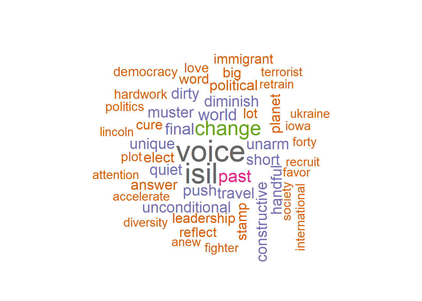
4 Visualization
Finally, visualize the result of the 50 most significant terms as Wordcloud. This can be realized simply by function of the package wordcloud. Additionally to the words and their weights (here we use likelihood values), we override default scaling and color parameters. Feel free to try different parameters to modify the wordcloud rendering.
require(wordcloud2)
top50 <- sort(logLikelihood, decreasing = TRUE)[1:50]
top50_df <- data.frame(word = names(top50), count = top50, row.names = NULL)
wordcloud2(top50_df, shuffle = F, size = 0.5)
5 Alternative reference corpora
Key term extraction cannot be done for single documents, but for entire (sub-)corpora. Depending on the comparison corpora, the results may vary. Instead of comparing a single document to a Wikipedia corpus, we now compare collections of speeches of a single president, to speeches of all other presidents.
For this, we iterate over all different president names using a for-loop. Within the loop, we utilize a logical vector (Boolean TRUE/FALSE values), to split the DTM into two sub matrices: rows of the currently selected president and rows of all other presidents. From these matrices our counts of target and comparison frequencies are created. The statistical computation of the log-likelihood measure from above, we outsourced into the function calculateLogLikelihood which we load with the source command at the beginning of the block. The function just takes both frequency vectors as input parameters and outputs a LL-value for each term of the target vector.
Results of the LL key term extraction are visualized again as a wordcloud. Instead of plotting the wordcloud into RStudio, this time we write the visualization as a PDF-file to disk into the wordclouds folder. After the for-loop is completed, the folder should contain 42 wordcloud PDFs, one for each president.
source("calculateLogLikelihood.R")

presidents <- unique(textdata$president)
for (president in presidents) {

  cat("Extracting terms for president", president, "\n")

  selector_logical_idx <- textdata$president == president

  presidentDTM <- targetDTM[selector_logical_idx, ]
  termCountsTarget <- colSums(presidentDTM)

  otherDTM <- targetDTM[!selector_logical_idx, ]
  termCountsComparison <- colSums(otherDTM)

  loglik_terms <- calculateLogLikelihood(termCountsTarget, termCountsComparison)

  top50 <- sort(loglik_terms, decreasing = TRUE)[1:50]

  fileName <- paste0("wordclouds/", president, ".pdf")
  pdf(fileName, width = 9, height = 7)
  wordcloud::wordcloud(names(top50), top50, max.words = 50, scale = c(3, .9), colors = RColorBrewer::brewer.pal(8, "Dark2"), random.order = F)
  dev.off()

}
6 Optional exercises
- Create a table (data.frame), which displays the top 25 terms of all speeches by frequency, tf-idf and log likelihood in columns.
##       word.frq  frq word.tfidf tfidf     word.ll   ll
## 1   government 6595    program  1007    congress 3085
## 2         make 5871    tonight   856  government 2732
## 3     congress 5040        job   768 unite_state 2016
## 4  unite_state 4518     mexico   679      nation 1685
## 5        state 4314    america   615     country 1511
## 6      country 4283  territory   551         law 1067
## 7         year 4132   economic   541       peace  960
## 8       people 3766       bank   537        duty  918
## 9        great 3555       cent   521       great  916
## 10 nation 3319 subject 513 interest 898- Create a wordcloud which compares Obama’s last speech with all his other speeches.
2020, Andreas Niekler and Gregor Wiedemann. GPLv3. tm4ss.github.io